This is the part 2 of my series on deep reinforcement learning. See part 1 “Demystifying Deep Reinforcement Learning” for an introduction to the topic.
The first time we read DeepMind’s paper “Playing Atari with Deep Reinforcement Learning” in our research group, we immediately knew that we wanted to replicate this incredible result. It was the beginning of 2014, cuda-convnet2 was the top-performing convolutional network implementation and RMSProp was just one slide in Hinton’s Coursera course. We struggled with debugging, learned a lot, but when DeepMind also published their code alongside their Nature paper “Human-level control through deep reinforcement learning”, we started working on their code instead.
The deep learning ecosystem has evolved a lot since then. Supposedly a new deep learning toolkit was released once every 22 days in 2015. Amongst the popular ones are both the old-timers like Theano, Torch7 and Caffe, as well as the newcomers like Neon, Keras and TensorFlow. New algorithms are getting implemented within days of publishing.
At some point I realized that all the complicated parts that caused us headaches a year earlier are now readily implemented in most deep learning toolkits. And when Arcade Learning Environment – the system used for emulating Atari 2600 games – released a native Python API, the time was right for a new deep reinforcement learning implementation. Writing the main code took just a weekend, followed by weeks of debugging. But finally it worked! You can see the result here: https://github.com/tambetm/simple_dqn
I chose to base it on Neon, because it has
- the fastest convolutional kernels,
- all the required algorithms implemented (e.g. RMSProp),
- a reasonable Python API.
I tried to keep my code simple and easy to extend, while also keeping performance in mind. Currently the most notable restriction in Neon is that it only runs on the latest nVidia Maxwell GPUs, but that’s about to change soon.
In the following I will describe
- how to install it
- what you can do with it
- how does it compare to others
- and finally how to modify it
How To Install It?
There is not much to talk about here, just follow the instructions in the README. Basically all you need are Neon, Arcade Learning Environment and simple_dqn itself. For trying out pre-trained models you don’t even need a GPU, because they also run on CPU, albeit slowly.
What You Can Do With It?
Running a Pre-trained Model
Once you have everything installed, the first thing to try out is running pre-trained models. For example to run a pre-trained model for Breakout, type:
./play.sh snapshots/breakout_77.pkl
Or if you don’t have a (Maxwell) GPU available, then you can switch to CPU:
./play.sh snapshots/breakout_77.pkl --backend cpu
You should be seeing something like this, possibly even accompanied by annoying sounds ![]()
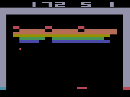
You can switch off the AI and take control in the game by pressing “m” on keyboard – see how long you last! You can give the control back to the AI by pressing “m” again.
It is actually quite useful to slow down the gameplay by pressing “a” repeatedly – this way you can observe what is really happening in the game. Press “s” to speed the game up again.
Recording a Video
Just as easily you can also record a video of one game (in Breakout until 5 lives are lost):
./record.sh snapshots/breakout_77.pkl
The recorded video is stored as videos/breakout_77.mov and screenshots from the game can be found in videos/breakout. You can watch an example video here:
Training a New Model
To train a new model, you first need an Atari 2600 ROM file for the game. Once you have the ROM, save it to roms folder and run training like this:
./train.sh roms/pong.rom
As a result of training the following files are created:
results/pong.csvcontains various statistics of the training process,snapshots/pong_<epoch>.pklare model snapshots after every epoch.
Testing a Model
During training there is a testing phase after each epoch. If you would like to re-test your pre-trained model later, you can use the testing script:
./test.sh snapshots/pong_141.pkl
It prints the testing results to console. To save the results to file, add --csv_file <filename> parameter.
Plotting Statistics
During and after training you might like to see how your model is doing. There is a simple plotting script to produce graphs from the statistics file. For example:
./plot.sh results/pong.csv
This produces the file results/pong.png.

By default it produces four plots:
- average score,
- number of played games,
- average maximum Q-value of validation set states,
- average training loss.
For all the plots you can see random baseline (where it makes sense) and result from training phase and testing phase. You can actually plot any field from the statistics file, by listing names of the fields in the --fields parameter. The default plot is achieved with --fields average_reward,meanq,nr_games,meancost. Names of the fields can be taken from the first line of the CSV file.
Visualizing the Filters
The most exciting thing you can do with this code is to peek into the mind of the AI. For that we are going to use guided backpropagation, that comes out-of-the-box with Neon. In simplified terms, for each convolutional filter it finds an image from a given dataset that activates this filter the most. Then it performs backpropagation with respect to the input image, to see which parts of the image affect the “activeness” of that filter most. This can be seen as a form of saliency detection.
To perform filter visualization run the following:
./nvis.sh snapshots/breakout_77.pkl
It starts by playing a game to collect sample data and then performs the guided backpropagation. The results can be found in results/breakout.html and they look like this:
There are 3 convolutional layers (named 0000, 0002 and 0004) and for this post I have visualized only 2 filters from each (Feature Map 0-1). There is also more detailed file for Breakout which has 16 filters visualized. For each filter an image was chosen that activates it the most. Right image shows the original input, left image shows the guided backpropagation result. You can think of every filter as an “eye” of the AI. The left image shows where this particular “eye” was directed to, given the image on the right. You can use mouse wheel to zoom in!
Because input to our network is a sequence of 4 grayscale images, it’s not very clear how to visualize it. I made a following simplification: I’m using only the last 3 screens of a state and putting them into different RGB color channels. So everything that is gray hasn’t changed over 3 images; blue was the most recent change, then green, then red. You can easily follow the idea if you zoom in to the ball – it’s trajectory is marked by red-green-blue. It’s harder to make sense of the backpropagation result, but sometimes you can guess that the filter tracks movement – the color from one corner to another progresses from red to green to blue.
Filter visualization is an immensely useful tool, you can immediately make interesting observations.
- The first layer filters focus on abstract patterns and cannot be reliably associated with any particular object. They often activate the most on score and lives, possibly because these have many edges and corners.
- As expected, there are filters that track the ball and the paddle. There are also filters that activate when the ball is about to hit a brick or the paddle.
- Also as expected, higher layer filters have bigger receptive fields. This is not so evident in Breakout, but can be clearly seen in this file for Pong. It’s interesting that filters in different layers are more similar in Breakout than in Pong.
How Does It Compare To Others?
There are a few other deep reinforcement learning implementations out there and it would be interesting to see how the implementation in Neon compares to them. The most well-known is the original DeepMind code published with their Nature article. Another maintained version is deep_q_rl created by Nathan Sprague from James Madison University in Virginia.
The most common metric used in deep reinforcement learning is the average score per game. To calculate it for simple_dqn I used the same evaluation procedure as in the Nature article – average scores of 30 games, played with different initial random conditions and an ε-greedy policy with ε=0.05. I didn’t bother to implement the 5 minutes per game restriction, because games in Breakout and Pong don’t last that long. For DeepMind I used the values from Nature paper. For deep_q_rl I I asked the deep-q-learning list members to provide the numbers. Their scores are not collected using exactly the same protocol (the particular number below was average of 11 games) and may be therefore considered a little bit inflated.
Another interesting measure is the number of training steps per second. DeepMind and simple_dqn report average number of steps per second for each epoch (250000 steps). deep_q_rl reports number of steps per second on the fly and I just used a perceived average of numbers flowing over the screen ![]() . In all cases I looked at the first epoch, where exploration rate is close to 1 and the results therefore reflect more of the training speed than the prediction speed. All tests were done on nVidia Geforce Titan X.
. In all cases I looked at the first epoch, where exploration rate is close to 1 and the results therefore reflect more of the training speed than the prediction speed. All tests were done on nVidia Geforce Titan X.
| Implemented in | Breakout average score | Pong average score | Training steps per second | |
| DeepMind | Lua + Torch | 401.2 (±26.9) | 18.9 (±1.3) | 330 |
| deep_q_rl | Python + Theano + Lasagne + Pylearn2 | 350.7 | ~20 | ~300 |
| simple_dqn | Python + Neon | 338.0 | 19.7 | 366 |
As it can be seen, in terms of speed simple_dqn compares quite favorably against the others. The learning results are not on-par with DeepMind yet, but they are close enough to run interesting experiments with it.
How Can You Modify It?
The main idea in publishing the simple_dqn code was to show how simple the implementation could actually be and that everybody can extend it to perform interesting research.
There are four main classes in the code: Environment, ReplayMemeory, DeepQNetwork and Agent. There is also main.py, that handles parameter parsing and instantiates the above classes, and the Statistics class that implements the basic callback mechanism to keep statistics collection separate from the main loop. But the gist of the deep reinforcement learning algorithm is implemented in the aforementioned four classes.
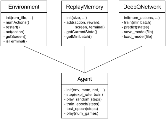
Environment
Environment is just a lightweight wrapper around the A.L.E Python API. It should be easy enough to add other environments besides A.L.E, for example Flappy Bird or Torcs – you just have to implement a new Environment class. Give it a try and let me know!
ReplayMemory
Replay memory stores state transitions or experiences. Basically it’s just four big arrays for screens, actions, rewards and terminal state indicators.
Replay memory is stored as a sequence of screens, not as a sequence of states consisting of four screens. This results in a huge decrease in memory usage, without significant loss in performance. Assembling screens into states can be done fast with Numpy array slicing.
Datatype for the screen pixels is uint8, which means 1M experiences take 6.57GB – you can run it with only 8GB of memory! Default would have been float32, which would have taken ~26GB.
If you would like to implement prioritized experience replay, then this is the main class you need to change.
DeepQNetwork
This class implements the deep Q-network. It is actually the only class that depends on Neon.
Because deep reinforcement learning handles minibatching differently, there was no reason to use Neon’s DataIterator class. Therefore the lower level Model.fprop() and Model.bprop() are used instead. A few suggestions for anybody attempting to do the same thing:
- You need to call Model.initialize() after constructing the Model. This allocates the tensors for layer activations and weights in GPU memory.
- Neon tensors have dimensions (channels, height, width, batch_size). In particular batch size is the last dimension. This data layout allows for the fastest convolution kernels.
- After transposing the dimensions of a Numpy array to match Neon tensor requirements, you need to make a copy of that array! Otherwise the actual memory layout hasn’t changed and the array cannot be directly copied to GPU.
- Instead of accessing single tensor elements with array indices (like tensor[i,j]), try to copy the tensor to a Numpy array as a whole with tensor.set() and tensor.get() methods. This results in less round-trips between CPU and GPU.
- Consider doing tensor arithmetics in GPU, the Neon backend provides nice methods for that. Also note that these operations are not immediately evaluated, but stored as a OpTree. The tensor will be actually evaluated when you use it or transfer it to CPU.
If you would like to implement double Q-learning, then this is the class that needs modifications.
Agent
Agent class just ties everything together and implements the main loop.
Conclusion
I have shown, that using a well-featured deep learning toolkit such as Neon, implementing deep reinforcement learning for Atari video games is a breeze. Filter visualization features in Neon provide important insights into what the model has actually learned.
While not the goal on its own, computer games provide an excellent sandbox for trying out new reinforcement learning approaches. Hopefully my simple_dqn implementation provides a stepping stone for a number of people into the fascinating area of deep reinforcement learning research.
Credits
Thanks to Ardi Tampuu, Jaan Aru, Tanel Pärnamaa, Raul Vicente, Arjun Bansal and Urs Köster for comments and suggestions on the drafts of this post.